RTOS Scheduler Simulator
What is this? This simulator visualizes how different Real-Time Operating System (RTOS) scheduling algorithms prioritize and execute tasks over time. Add your custom tasks below, select a scheduling algorithm, and run the simulation to generate an interactive chart.
Supported Algorithms
- EDF (Earliest Deadline First): Dynamic priority. The scheduler always chooses the ready task with the closest absolute deadline. Preemptive.
- RM (Rate Monotonic): Static priority. Tasks with shorter periods are assigned higher priority. It is optimal for periodic tasks. Preemptive.
- FCFS (First Come First Serve): Non-preemptive. The scheduler simply executes tasks in the exact order they arrive, ignoring deadlines and periods.
RTOS Scheduling Algorithms Summary
| Algorithm | Type | Task Environment / Constraints | Principle | Complexity | Optimality | Schedulability Guarantee |
|---|---|---|---|---|---|---|
| EDD (Jackson '55) |
Aperiodic | Sync activation, Independent 1|sync|Lmax |
Earliest Due Date | O(n log n) | Optimal | ∑k=1i Ck < di |
| EDF (Horn '74) |
Aperiodic | Async activation, Preemptive, Independent 1|preem|Lmax |
Earliest Deadline First | O(n2) | Optimal | ∑k=1i ck(t) < di |
| Tree Search (Bratley '71) |
Aperiodic | Async activation, Non-preemptive, Independent | Tree Search | O(n · n!) | Optimal | - |
| LDF (Lawler '73) |
Aperiodic | Sync activation, Precedence (DAG) 1|(prec,sync)|Lmax |
Latest Deadline First | O(n2) | Optimal | - |
| EDF* (Chetto '90) |
Aperiodic | Async preemptive, Precedence (DAG) 1|(prec,sync)|Lmax |
Modified EDF (Alters aj, dj) | O(n2) | Optimal | - |
| Spring (Stankovic '87) |
Aperiodic | Async non-preemptive, Precedence (DAG) | Heuristic Search | O(n2) | Heuristic | - |
| RMA (Liu & Layland '73) |
Periodic | Static Priority, di = Ti 1|fixed priority|∑ Ui |
Rate Monotonic | - | Optimal | U = ∑ (Ci/Ti) ≤ n(21/n-1) |
| DMA (Leung & Whitehead '82) |
Periodic | Static Priority, di ≤ Ti 1|(fixed priority,Di ≤ Ti)|Lmax |
Deadline Monotonic | - | Optimal | Di ≥ Ci + Ii |
| EDF (Priority) (Liu & Layland '73) |
Periodic | Dynamic Priority, di = Ti 1|dyn priority|Cmax |
Earliest Deadline First | - | Optimal | U = ∑ (Ci/Ti) ≤ 1 |
| PDA EDF (Baruah et al. '90) |
Periodic | Dynamic Priority, di ≤ Ti 1|dyn priority|Cmax |
Processor Demand Analysis | - | Optimal | L ≥ ∑ (⌊(L-Di)/Ti⌋ + 1)Ci |
| Polling Server (PS) | Mixed | Static Priority Server (RM) + Aperiodic requests | Periodic capacity Cs, fully discharges if queue is empty at start | - | Heuristic | Ups ≤ n [ (2 / (Us + 1))1/n - 1 ] |
| Deferrable Server (DS) | Mixed | Static Priority Server (RM) + Aperiodic requests | Maintains capacity Cs throughout the server period | - | Heuristic | Uds ≤ n [ ((Us + 2) / (2Us + 1))1/n - 1 ] |
| Total Bandwidth Server (TBS) | Mixed | Dynamic Priority Server (EDF) + Aperiodic requests | Deadlines assigned dynamically to not exceed bandwidth: dk = max(rk, dk-1) + Ck / Us | - | Heuristic | Up + Us < 1 |
RTOS Scheduling Literature Review
1. Introduction
1.1 Terminology
- Task: A process in the Real Time environment
- Active Task: A task that can be executed by the CPU
- Ready Task: a task waiting in the queue, waiting for the CPU
- Running Task: A task that is currently executed by the CPU
- Scheduling Algorithm: Algorithm that defines the task execution order
1.2 Scheduling
Given a set of tasks J = {J1, &dots;, Jn}, a schedule is an assignment of tasks to the processor so that each task is executed until completion.
Formally a schedule is:
s : ℝ+ → ℕ such that ∀ t ∈ ℝ+, ∃ t1, t2 ∈ ℝ+ | ∀ t' ∈ [t1, t2), s(t) = s(t')
1.3 Properties
- schedulability: A set of task is schedulable if there exists at least one algorithm that can produce a feasible schedule
- feasibility: A schedule is feasible if all task can be completed according to a set of specified constraints
1.4 Task Characterization
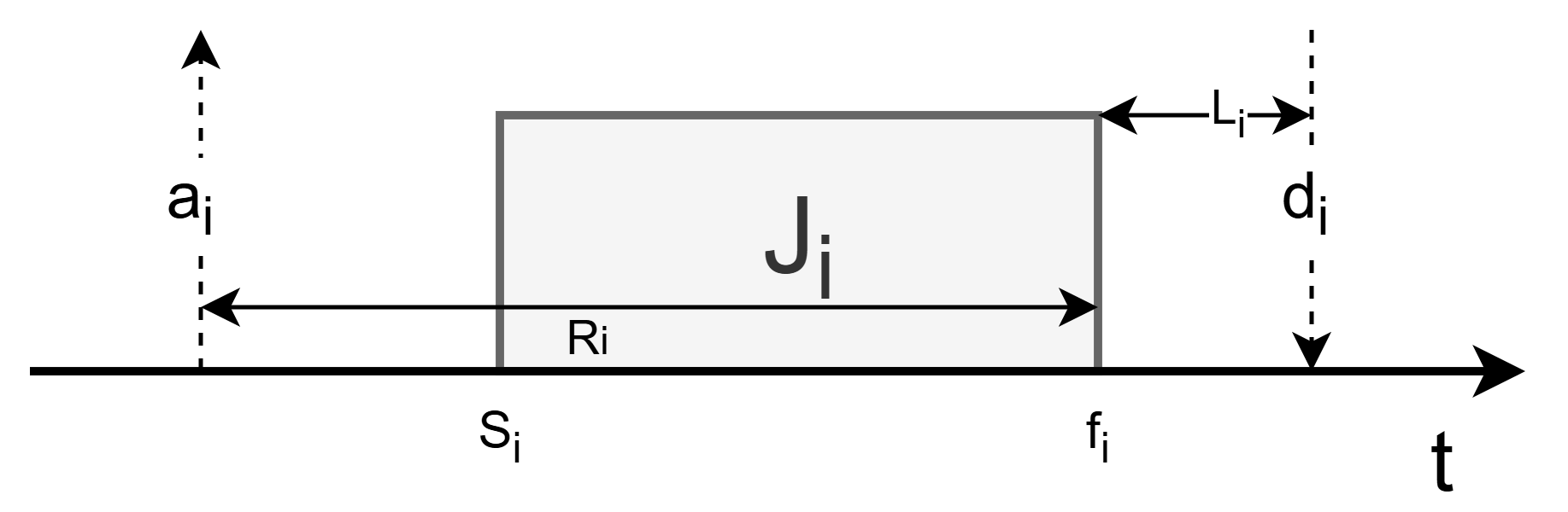
The tasks have different properties, that are used to schedule them, accordingly to the scheduling algorithm. Given the task Ji:
- Parameters
- Arrival time ai: the time at which the task is ready to be executed
- Period time Ti: the recurring time at which the task is ready to be executed
- Computation time Ci: the time needed to execute the task (with no interruption)
- Deadline di: the time before which the task needs to conclude its execution
- Start time si: the time at which the task is starts running
- Finish time fi: the time at which the task finished its execution
- Metrics
- Response Time Ri = fi - ai: the interval of time from where the task is arrived to when the task finished its execution
- Lateness Li = fi - di: the residual time between the execution conclusion and the deadline
- Slack time Xi = di - ai - Ci: maximum time a task can be delayed to complete within its deadline
1.5 Constraints
The feasibility constraints for the schedulability are:
- Timing: the task ends their execution before their deadline, the missed deadline is divided into three classes: Hard (cause catastrophic consequence) , Soft (cause performance degradation) or Firm (causes no harm, but the result is useless)
- Precedence: the tasks are executed following precedence rule
- Resource: the task can only access the available resource (those not locked by other tasks)
1.5.1 Task Activation
The task are infinite sequence of identical activities (instances)
- Time activation
- Periodic Task: activated each period Ti
- Event activation
- Aperiodic Task: activation is not known and can vary over time
- Sporadic Task: is an aperiodic task than might activate again after a fixed inter-arrival time
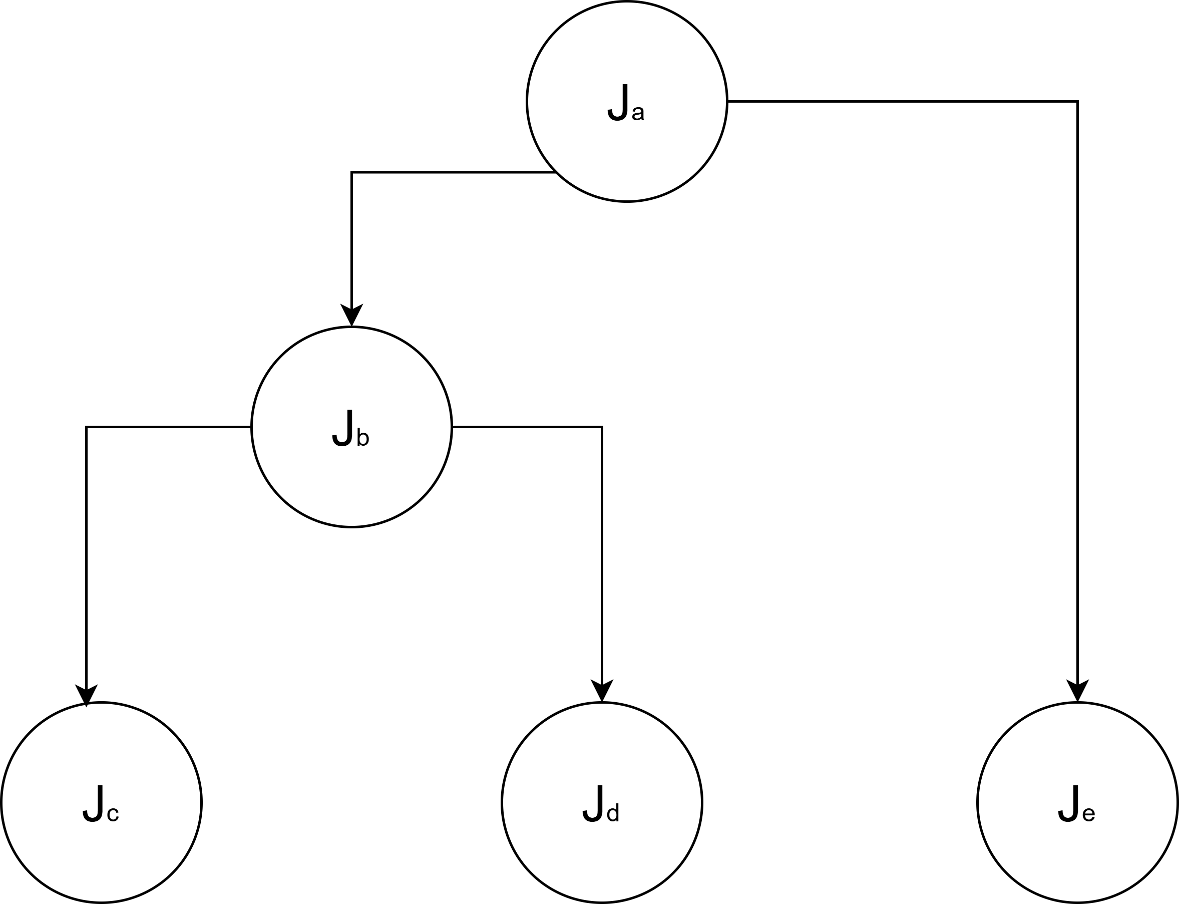
1.5.2 Precedence Constraints
The execution order of the tasks has to respect a precedence relation, usually expressed with a Direct Access Graph (DAG) and are denoted as:
- Predecessor Ja < Jc: the task Ja is a predecessor of the task Jc
- Immediate predecessor Ja → Jb: the task Ja is a immediate predecessor of the task Jb
1.5.3 Resource Constraints
Resource access is particularly critical for Real Time OS, classical structure like semaphores can't be used
2. Scheduling Problem
The scheduling is a nondeterministic polynomial (NP) complete problem
2.1 Problem Definition
Given
- a set of tasks J = {J1,...,Jn} with their constraints
- a set of processors P = {P1,...,Pn}
- a set of resources R = {R1,...,Rn}
- a set of precedence specified with a DAG
Scheduling is the process of assigning a processor Pj and resource Rk to a task Ji under their constraints
2.2 Scheduler Classification
Real-time scheduling disciplines are typically characterized by four primary design dimensions:
- Preemption strategy
- Preemptive: the current task can be interrupted
- Non-preemptive: once a task starts, it runs to completion without interruption
- Priority assignment
- Static: priorities are assigned before activation
- Dynamic: priorities can change during runtime
- Decision timing
- Off-line: the schedule is pre-computed before the system start
- On-line: the schedule is made at run time as the tasks arrive
- Optimality
- Optimal: Guaranteed to find a feasible schedule if one exists
- Heuristic: Uses rules of thumb for good enough results
2.3 Guaranteed Scheduling
Since Hard Real Time system require feasibility of the schedule, it must be guaranteed in advance. Given this we can define two type of scheduler:
- Static offline scheduling: Decisions are made at compile-time and requires almost no CPU overhead at runtime but offers zero flexibility
- Dynamic online scheduling: Decisions are made at run-time, feasibility is still guaranteed in advance by proving that in the worst case assumption, the mathematical properties of the algorithm ensure it
2.4 Scheduling Metrics
Scheduling metrics are essential tools used to evaluate, verify, and optimize the performance of a real-time system. While the primary goal of hard real-time systems is to ensure all deadlines are met, metrics provide the quantitative data needed to prove this will happen before the system even runs. Generally, a mix of those is used.
- Average response time: no information about deadline satisfaction
t̅r = (1/n) ∑i=1n (fi - ai) - Total completion time: no information about deadline satisfaction
tc = maxi(fi) - mini(ai) - Weighted sum of completion times:
tw = ∑i=1n wi fi - Maximum lateness: minimizing maximum lateness does not minimize the number of tasks that miss deadlines
Lmax = maxi(fi - di) - Maximum number of late tasks:
Nlate = ∑i=1n miss(fi)
where miss(fi) = 0 if fi ≤ di, and 1 otherwise.
2.5 Scheduling Anomalies
Given a set of task with feasible scheduling, following the problem definition, the optimization of some of it's parameters (like increasing the number of processors, decreasing the computation time or weakening the precedence constraints) can produce an unfeasible scheduling, as Ronald L. Graham demonstrated in 1966
2.6 Problem Classification
To make the problem more tractable a classification is needed, where different algorithms solve different problems.
Ronald Graham, Eugene Lawler, Jan Karel Lenstra, and Alexander Rinnooy Kan proposed in 1979 a theoretical categorization of the scheduling algorithm, using the following three field annotation (α, β, γ)
- Machine environment (α): environment on which the task set has to be scheduled (usually the number of processors)
- Job description (β): task and resource characteristics (like preemption, precedence, synchronization, activation, ...)
- Objective criterion (γ): cost function to be optimized
3. Aperiodic Task Scheduling
Based on tasks Job description β: (synchronous or asynchronous activation, independent or precedence dependent, preemptive or non-preemptive), they can be solved with the following algorithms:
| sync. activation | preemptive async. activation |
non-preemptive async. activation |
|
|---|---|---|---|
| independent | EDD (Jackson '55) O(n log n) Optimal |
EDF (Horn '74) O(n2) Optimal |
Tree search (Bratley '71) O(n · n!) Optimal |
| precedence constraints |
LDF (Lawler '73) O(n2) Optimal |
EDF* (Chetto et al. '90) O(n2) Optimal |
Spring (Stankovic & Ramamritham '87) O(n2) Heuristic |
3.1 EDD Algorithm
The EDD algorithm, invented by Jackson in 1955, solves 1|sync|Lmax:
- Task set: J = {Ji (Ci,di) | i=1,...,n}
- Principle: Earliest Due Date (complexity O(n log n))
- Optimality: Optimal, no feasible schedule guarantee
- Schedulability guarantee: ∑k=1i Ck < di, ∀ i = 1,...,n with task listed with increasing deadlines
where, in the three field notation
- α = 1: 1 processor
- β = sync: all tasks arrive at the same time (non-preemptive) and are implicitly independent (no precedence constraints nor shared resources)
- γ = Lmax: minimize the number of late tasks
3.2 EDF Algorithm
The EDF algorithm, invented by Horn in 1974, solves 1|preem|Lmax:
- Task set: J = {Ji (Ci,ai,di) | i=1,...,n}
- Principle: Earliest Deadline first (complexity O(n2))
- Optimality: Optimal, no feasible schedule guarantee
- Schedulability guarantee: ∑k=1i ck(t) < di, ∀ i = 1,...,n with task listed with increasing deadlines and ci the remaining worst case execution time (WCET) of the task Ji
where, in the three field notation
- α = 1: 1 processor
- β = preem: tasks arrive at different time (preemptive),
- γ = Lmax: minimize the number of late tasks and are implicitly independent (no precedence constraints nor shared resources)
3.3 LDF Algorithm
The LDF algorithm, invented by Lawler in 1973, solves 1|(prec,sync)|Lmax:
- Task set: J = {Ji (Ci,ai,di) | i=1,...,n} with DAG constraints
- Principle: Latest Deadline first (complexity O(n2))
- Optimality: Optimal, no feasible schedule guarantee
- Schedulability guarantee: -
where, in the three field notation
- α = 1: 1 processor
- β = (prec,sync): all tasks arrive at the same time (non-preemptive) and are dependent, following the DAG
- γ = Lmax: minimize the number of late tasks and are implicitly independent (no precedence constraints nor shared resources)
3.4 LDF* Algorithm
The EDF* algorithm, invented by Chetto in 1990, solves 1|(prec,sync)|Lmax:
- Task set: J = {Ji (Ci,ai,di) | i=1,...,n} with DAG constraints
- Principle: Modified Latest Deadline first, change the tasks parameters and makes them independent by exploiting the DAG, given Jj → Jk:
- task cannot start before its predecessors: aj = max(aj, ak - Ck)
- cannot preempt their successor: dj = max(dj, dk - Ck)
- Optimality: Optimal, no feasible schedule guarantee
- Schedulability guarantee: -
where, in the three field notation
- α = 1: 1 processor
- β = (prec,sync): all tasks arrive at the same time (non-preemptive) and are dependent, following the DAG
- γ = Lmax: minimize the number of late tasks and are implicitly independent (no precedence constraints nor shared resources)
4. Periodic Task Scheduling
The periodic tasks are the majority of the task type usually executed in RTOS. Based on tasks Job description β, they can be solved with the following algorithms:
| di = Ti | di ≤ Ti | |
|---|---|---|
| Static Priority |
RMA Processor utilization approach ∑i=1n (Ci / Ti) ≤ n(21/n - 1) |
DMA Response time approach ∀ i, Ri = Ci + ∑j ∈ hp(i) ⌈ Ri / Tj ⌉ Cj ≤ Di |
| Dynamic Priority |
EDF Processor utilization approach ∑i=1n (Ci / Ti) ≤ 1 |
EDF Processor demand approach ∀ L > 0, L ≥ ∑i=1n (⌊ (L - Di) / Ti ⌋ + 1) Ci |
4.1 Cyclic Executive Scheduling
Cyclic Executive Scheduling is a deterministic, time-triggered scheduling approach where tasks are executed in a fixed, repeating sequence called a major cycle. While being logically simple, might be difficult to construct (bin packing problem)
The tasks are mapped in a set of minor cycles, that than constitute the major cycle
4.2 Schedulability guarantee
The schedulability guarantee of the following algorithm is based on two different factors:
- processor utilization factor
- worst case response time factor
4.2.1 Processor utilization factor
Given a set of periodic task Γ, the utilization factor U is the fraction of processor time spent in the execution of the task set
UΓ = ∑i=1,...,n (Ci / Ti)
The schedulability test is sufficient, but not necessary:
- Schedulable: UΓ ≤ Ulub(A)
- Maybe schedulable: UΓ > Ulub(A)
- Not schedulable: UΓ > 1
where Ulub(A) is the least upper bound of the utilization factor of a given algorithm A
Ulub(A) = min(Ulub(A, Γ)) ∀ Γ
4.2.2 Response time factor
The worst case response time analysis is sufficient and necessary condition to determine the schedulability of a task set.
Ri = Ci + Ii
where Ii = ∑j ∈ hp(i) ⌈ Ri / Tj ⌉ Cj is the maximum interference that a task can experience.
Then the scheduling is granted if and only if Ri > di ∀ i.
4.3 RM Algorithm
The RM algorithm, invented by Liu and Layland in 1973, solves 1|fixed priority|∑ Ui:
- Task set: J = {Ji (Ci,ai,di) | i=1,...,n}
- Principle: Rate Monotonic, priorities are assigned according to request rates
- Optimality: Optimal, no feasible schedule guarantee
- Schedulability guarantee:
- WCRT factor: Ri = Ci + Ii
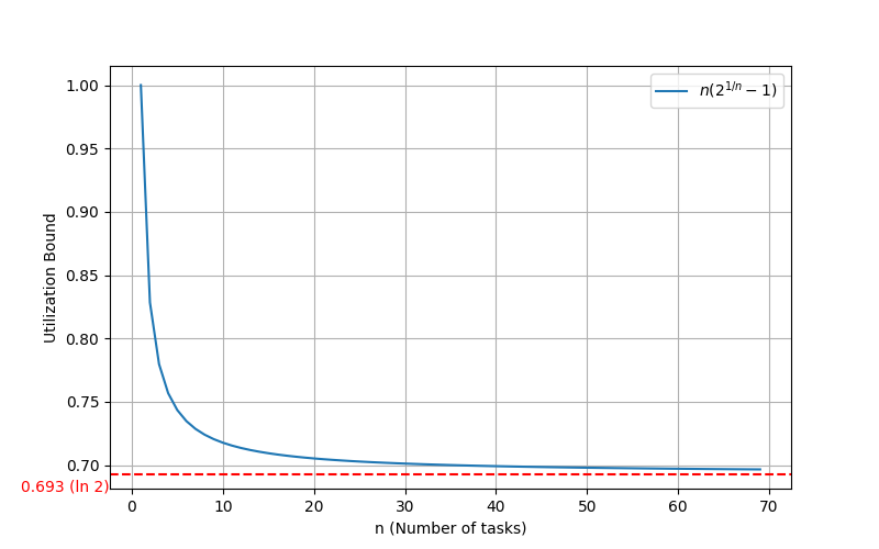
- U factor: Ulub = ∑i=1n (Ci / Ti) ≤ n(21/n - 1)
where, in the three field notation
- α = 1: 1 processor
- β = (priority): tasks have fixed priority (preemptive)
- γ = ∑ Ui: ensure that the process utilization is within the schedulable bound
4.4 Priority EDF Algorithm
The EDF priority based algorithm, invented by Liu and Layland in 1973, solves 1|dyn priority|Cmax:
- Task set: J = {Ji (Ci,ai,di) | i=1,...,n}
- Principle: Earliest Deadline first where task with earlier deadline are assigned to higher priorities
- Optimality: Optimal, no feasible schedule guarantee
- Schedulability guarantee: Ulub = ∑i=1n (Ci / Ti) ≤ 1 (necessary and sufficient)
where, in the three field notation
- α = 1: 1 processor
- β = (dyn priority): tasks have dynamic priority (preemptive)
- γ = Cmax: minimizes the total computation time
4.5 DM Algorithm
The DM algorithm, invented by Leung and Whitehead in 1982, solves 1|(fixed priority, Di ≤ Ti)|Lmax:
- Task set: J = {Ji (Ci,ai,di) | i=1,...,n}
- Principle: Deadline Monotonic, priorities are assigned according to request rates
- Optimality: Optimal, no feasible schedule guarantee
- Schedulability guarantee: Di ≥ Ci + Ii, with Ii maximum interference that a task can experience.
where, in the three field notation
- α = 1: 1 processor
- β = (priority): tasks have fixed priority (preemptive)
- γ = Lmax: ensure that all the tasks meet their deadline
4.6 PDA EDF Algorithm
The Processor Demand Analysis EDF algorithm, invented by Baruah, Rosier and Howell in 1990, solves 1|dyn priority|Cmax:
- Task set: J = {Ji (Ci,ai,di) | i=1,...,n}
- Principle: Earliest Deadline first where task with earlier deadline are assigned to higher priorities
- Optimality: Optimal, no feasible schedule guarantee
- Schedulability guarantee: L ≥ ∑i=1n (⌊ (L - Di) / Ti ⌋ + 1) Ci ∀ L > 0, where L is the interval length
where, in the three field notation
- α = 1: 1 processor
- β = (dyn priority): tasks have dynamic priority (preemptive)
- γ = Cmax: minimizes the total computation time
4.7 Comparison: RM vs EDF
RM characteristics
- Simple to implement
- U < 69%
- During overload, lower priority task blocked
- Leaves time for others tasks (useful in mixed tasks environment)
EDF characteristics (corrected title based on context)
- Hard to implement
- U ≅ 100%
- During overload, lower priority task not blocked
5. Mixed Task Scheduling
Mixed-task scheduling deals with systems where different types of tasks (periodic, sporadic, and aperiodic) must coexist on the same processor without compromising the deadlines of the critical tasks.
There are three main different approach to handle mixed tasks:
- Immediate service: aperiodic requests are served as soon as arrived, postponing periodic tasks
- Background scheduling:
- Periodic task: assigned to high priority queue and scheduled with RM
- Aperiodic task: assigned to high priority queue and scheduled with FCFS (first come, first served)
- Aperiodic server (static or dynamic): uses a priority server that handles the aperiodic tasks as aperiodic ones
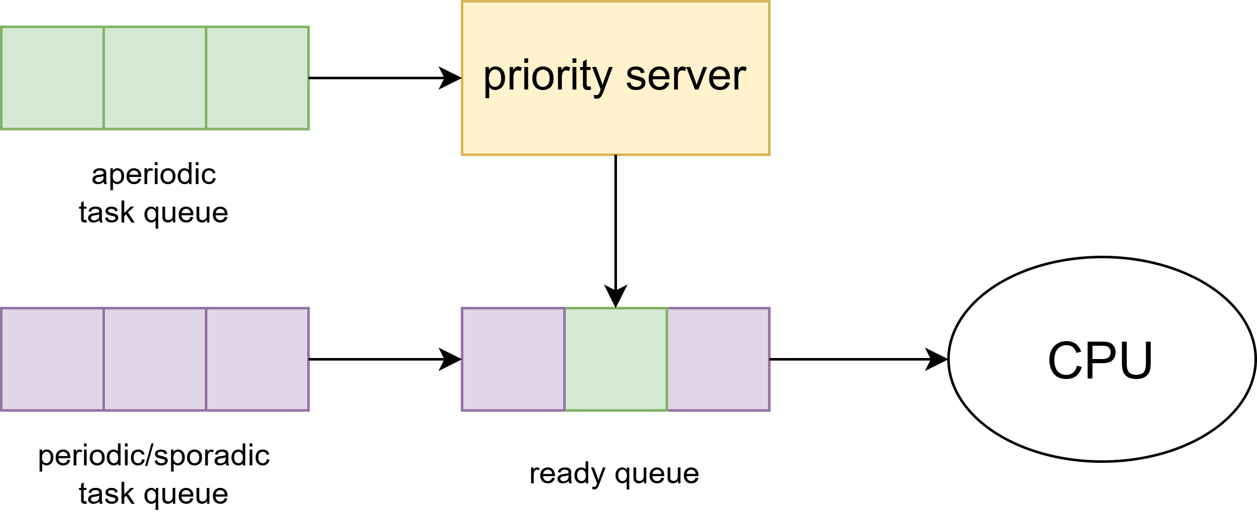
Figure 4: Priority server approach
5.1 Static Priority Server
Static priority server insert aperiodic tasks in the ready queue, mixing with periodic tasks, then apply RM as for periodic tasks.
There are different type of static priority server:
- Polling Server
- Deferrable Server
- Priority Exchange
- Sporadic Server
- Slack Stealing
5.1.1 Polling Server
The aperiodic tasks accumulate in the queue and at the start of the priority server period, it sets its capacity Cs to maximum, then
- Aperiodic task pending: the server loads the aperiodic tasks to maximum its capacity Cs (the capacity might be not fully used)
- Aperiodic task queue empty: the server loads no aperiodic tasks and discharge its capacity to 0
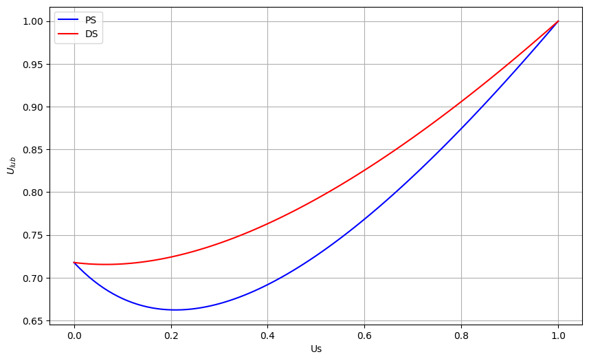
The schedulability analysis is computed using the Utilization Factor (PS+RM):
Ups ≤ n [ (2 / (Us + 1))1/n - 1 ]
5.1.2 Deferrable Server
The deferrable server is similar to the polling server, but handles the capacity discharge differently: as soon as an aperiodic tasks arrived, it is immediately moved to the priority server, until it hits the maximum capacity.
The schedulability analysis is computed using the Utilization Factor (DS+RM):
Uds ≤ n [ ((Us + 2) / (2Us + 1))1/n - 1 ]
5.1.3 PS and DS comparison
By analyzing their utilization factor, we can find out that:
- Invasive behavior of the DS causes lower schedulability bound for periodic tasks
- DS is more responsive than PS but decreases the utilization bound
5.2 Dynamic Priority Server
Dynamic priority server adapts the static priority server approach using EDF:
- the deadline of the aperiodic tasks is assigned in order to not exceed the given bandwidth Us: dk = max(rk, dk-1) + Ck / Us
- the periodic and aperiodic tasks are mixed and scheduled with EDF
There are different type of static priority server:
- Dynamic polling server
- Dynamic deferrable server
- Dynamic sporadic server
- Total bandwidth server
- Constant bandwidth server
5.2.1 Total Bandwidth Server
The schedulability analysis is computed using the Utilization Factor (TBS+EDF):
Up + Us < 1